A Geometric Perspective On Your Differential Equation, Part 1

While waiting for my eggs to hard-boil, I thought I’d introduce my readers (all of you) to the dangerously delightful world of Algebrential GeomAppliedMathFunctionalAnaletry. I say dangerously delightful because, due to the extremely broad thinking required, very few people do math this way. Don’t say I didn’t warn you.

Say you have a simple algebraic equation, like . Its solutions trace out a locus in , do they not? So we can visualize an equation, a sentence of numbers, functions, and variables, by thinking of the locus of its solutions in — its graph with respect to some coordinate axes.

Meditate on this for a moment. I want you to really, really hardcore appreciate that we have a way of visualizing algebraic equations that’s so simple we can teach it to middle schoolers. Stop taking this power for granted. Sing Hallelujah and praise the name of Descartes!

So now we’ve got our example-gadget, , and we want to graph it. All we need is a basis. I choose… ! I’ve pulled the old switcheroo: we’re no longer in , we’re in ; is now some kind of forcing function; and our solutions , while still points in the space, are now solutions ! Who saw that coming?

Don’t be daunted by the prospect of graphing something in an infinite-dimensional space. If you’re graphing any equation as a line, and then you add more dimensions to your space, your graph merely becomes a -dimensional surface rather than a line. Just as we think of the point as a list of coefficients for the etc. basis vectors of (the point’s “coordinates”), we will think of a function as a list of its Fourier coefficients. These lists will tell us how far apart two functions are, to give us a sense of geometry. It doesn’t matter that it’s a function space – you can still draw stuff in it.

Now, there are some operators we can apply to algebraic equations. Only usually we don’t call them operators; we call them functions. Things like sine, cosine, ln, exp, et cetera. The graph of 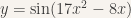 looks a lot different from the graph of , but is still totally within the realm of drawability. Well, there’s one operator I want to talk about that we actually do call an operator, and that’s the differential operator. The graph of  also looks pretty different from that of . But y’know what? We can think of the graph of a derivative in the same way as the graph of a derivative in – we took an equation whose solutions we could graph, we applied an operator to it, and now we have another equation whose solutions we can graph.

To recap: Thanks to our venerated hero René Descartes, we know that an equation traces out a locus of its solutions in some solution space, no matter what that space is, as long as it’s got a basis out of which we can make coordinates.